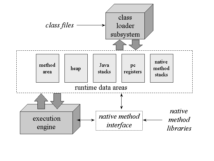
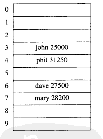
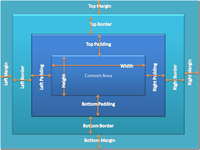
PC register - If that method is not native , the pc register contains the address of the Java Virtual Machine instruction currently being executed.
Java stacks - A Java Virtual Machine stack is analogous to the stack of a conventional language such as C: it holds local variables and partial results, and plays a part in method invocation and return.
Heap - The heap is the run-time data area from which memory for all class instances and arrays is allocated.
Method area - The method area is analogous to the storage area for compiled code of a conventional language or analogous to the “text” segment in an operating system process. It stores per-class structures such as the run-time constant pool, field and method data, and the code for methods and constructors, including the special methods used in class and instance initialization and interface initialization.
Native method stacks - An implementation of the Java Virtual Machine may use conventional stacks, colloquially called “C stacks,” to support native methods (methods written in a language other than the Java programming language). Native method stacks may also be used by the implementation of an interpreter for the Java Virtual Machine’s instruction set in a language such as C。
@FunctionalInterface interfaceCalculator{ intcal(int a, int b); }
publicclassHelloWorld{ publicstaticvoidmain(String[] args){ Calculator c = (a, b) -> a + b; System.out.println(c.cal(1, 2)); c = (a, b) -> a * b; System.out.println(c.cal(1, 2)); } }
Lambda 形式
Lambda 表达式的基本形式如下所示:
1
(argument list) -> code
下面是一个例子:
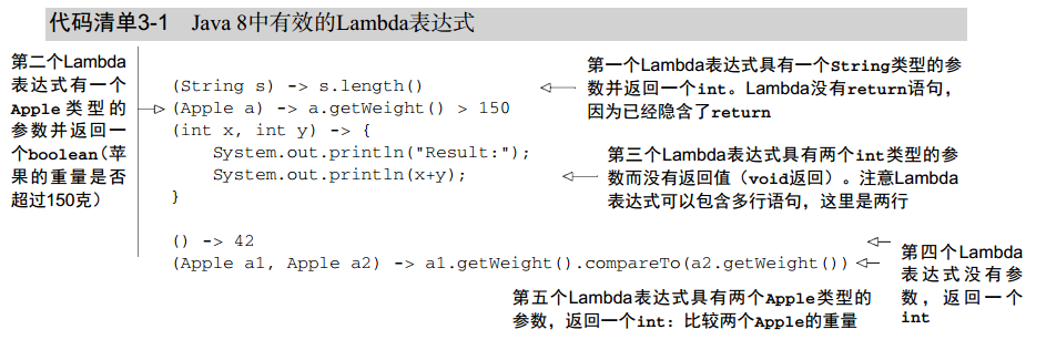
如上所示: Lambda 表达式包含三个部分:
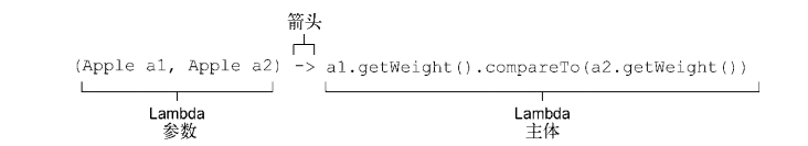
参数列表(A list of parameters) - 上图中为 (Apple a1, Apple a2)
箭头(An arrow) - 把参数列表和 Lambda 主体分隔开
Lambda 主体(The body of the lambda) - 上图中为 a1.getWeight().compareTo(a2.getWeight()),该 Lambda 主体会返回 compareTo 的结果。
@FunctionalInterface interfaceCalculator{ intcal(int a, int b); }
下面是使用 lambda 表达式以及匿名类来创建 Calculator 对象的示例代码。在下面的代码中对象 c 和 c2 的实现是等价的。
1 2 3 4 5 6 7 8 9 10
publicvoiddemo(){ Calculator c = (int a, int b) -> a + b;
Calculator c2 = new Calculator() { @Override publicintcal(int a, int b){ return a + b; } }; }
从上面的例子中,我们可以看到 Lambda 表达式 是和函数式接口中的 抽象方法 进行匹配的,其中 Lambda 表达式中参数匹配 cal 方法的参数,Lambda body 的内容作为抽象方法的具体实现,Lambda body 的计算值作为方法的返回值。这也是为什么要求函数式接口只能有一个抽象方法的原因。
@FunctionalInterface interfaceThrowExceptionInterface{ voidrun(int a, int b); }
publicclassLambdaTest{
publicvoidthrowException(){ // 这里编译时会报 Unhandled Exception:java.io.Exception ThrowExceptionInterface t = (int a, int b) -> { thrownew IOException(); }; } }
其实也很好理解,Lambda body 中的内容会作为抽象方法的具体实现,在方法中抛出了异常但是方法声明中却没有相关的异常声明,编译器肯定要报错的。
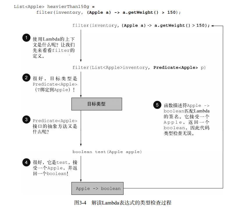
Lambda 表达式会赋值给 Calculator 对象,那么该 Lambda 表达式对应的目标类型就是 Calculator 接口,该接口中的 cal 方法对应的函数描述符为 (int, int) -> int,这个和 (int a, int b) -> a + b 可以匹配,这样就完成了类型检查。下图是一个完整的例子:
/** * Represents a predicate (boolean-valued function) of one argument. */ @FunctionalInterface publicinterfacePredicate<T> {
/** * Evaluates this predicate on the given argument. * * @param t the input argument * @return true if the input argument matches the predicate, * otherwise false */ booleantest(T t);
/** * Returns a composed predicate that represents a short-circuiting logical * AND of this predicate and another. When evaluating the composed * predicate, if this predicate is false, then the other * predicate is not evaluated. */ default Predicate<T> and(Predicate<? super T> other){ Objects.requireNonNull(other); return (t) -> test(t) && other.test(t); }
/** * Returns a predicate that represents the logical negation of this * predicate. */ default Predicate<T> negate(){ return (t) -> !test(t); }
/** * Returns a composed predicate that represents a short-circuiting logical * OR of this predicate and another. When evaluating the composed * predicate, if this predicate is true, then the other * predicate is not evaluated. */ default Predicate<T> or(Predicate<? super T> other){ Objects.requireNonNull(other); return (t) -> test(t) || other.test(t); }
/** * Returns a predicate that tests if two arguments are equal according * to {@link Objects#equals(Object, Object)}. */ static <T> Predicate<T> isEqual(Object targetRef){ return (null == targetRef) ? Objects::isNull : object -> targetRef.equals(object); } }
我们看到在 Predicate 类中,除了 test 方法,还定义了三个 default 方法,and, or 和 negate,它们分别对应逻辑运算中的与(&&)、或(||)、非(!)操作。通过这三个方法,我们可以构造更复杂的 predicate 表达式:
1 2 3 4 5 6 7 8
publicvoidtestPredicate(){ String text = "111"; Predicate<String> a = s - > s != null; Predicate<String> b = s - > s.length() > 3; System.out.println(judge(text, a.and(b))); System.out.println(judge(text, a.negate())); System.out.println(judge(text, a.or(b))); }
对应的输出结果为:
1 2 3
false false true
另外 and 和 or 方法是按照在表达式链中的位置,从左向右确定优先级的。因此 a.or(b).and(c) 可以看作 (a || b) && c。
/** * Represents a predicate (boolean-valued function) of two arguments. This is * the two-arity specialization of {@link Predicate}. */ @FunctionalInterface publicinterfaceBiPredicate<T, U> {
booleantest(T t, U u);
default BiPredicate<T, U> and(BiPredicate<? super T, ? super U> other){ Objects.requireNonNull(other); return (T t, U u) -> test(t, u) && other.test(t, u); }
/** * Represents an operation that accepts a single input argument and returns no * result. Unlike most other functional interfaces, Consumer is expected * to operate via side-effects. */ @FunctionalInterface publicinterfaceConsumer<T> {
/** * Performs this operation on the given argument. * * @param t the input argument */ voidaccept(T t);
/** * Returns a composed Consumer that performs, in sequence, this * operation followed by the after operation. If performing either * operation throws an exception, it is relayed to the caller of the * composed operation. If performing this operation throws an exception, * the after operation will not be performed. */ default Consumer<T> andThen(Consumer<? super T> after){ Objects.requireNonNull(after); return (T t) -> { accept(t); after.accept(t); }; } }
publicvoidtestConsume(){ StringBuilder builder = new StringBuilder(); Consumer <StringBuilder> a = s -> s.append("abcd"); Consumer <StringBuilder> b = s -> s.reverse(); Consumer <StringBuilder> c = s -> s.append("1234"); consume(builder, a.andThen(b).andThen(c)); System.out.println(builder.toString()); }
/** * Represents an operation that accepts two input arguments and returns no * result. This is the two-arity specialization of Consumer. * Unlike most other functional interfaces, BiConsumer is expected * to operate via side-effects. */ @FunctionalInterface publicinterfaceBiConsumer<T, U> {
voidaccept(T t, U u);
default BiConsumer<T, U> andThen(BiConsumer<? super T, ? super U> after){ Objects.requireNonNull(after);
/** * Represents a function that accepts one argument and produces a result. */ @FunctionalInterface publicinterfaceFunction<T, R> {
/** * Applies this function to the given argument. */ R apply(T t);
/** * Returns a composed function that first applies the before * function to its input, and then applies this function to the result. * If evaluation of either function throws an exception, it is relayed to * the caller of the composed function. */ default <V> Function<V, R> compose(Function<? super V, ? extends T> before){ Objects.requireNonNull(before); return (V v) -> apply(before.apply(v)); }
/** * Returns a composed function that first applies this function to * its input, and then applies the after function to the result. * If evaluation of either function throws an exception, it is relayed to * the caller of the composed function. */ default <V> Function<T, V> andThen(Function<? super R, ? extends V> after){ Objects.requireNonNull(after); return (T t) -> after.apply(apply(t)); }
/** * Returns a function that always returns its input argument. */ static <T> Function<T, T> identity(){ return t -> t; } }
publicvoidtestFunction(){ Function<Integer, Integer> f = x -> x + 1; Function<Integer, Integer> g = x -> x * 2; int i = func(1, f.andThen(g)); // 输出 4 System.out.println(i);
i = func(1, f.compose(g)); // 输出 3 System.out.println(i); }
UnaryOperator
UnaryOperator 是一种特殊的 Function,表示操作数和返回值是同一种类型,函数描述符为 T -> T。下面是该接口的定义:
1 2 3 4 5 6 7 8 9 10 11 12 13 14 15
/** * Represents an operation on a single operand that produces a result of the * same type as its operand. This is a specialization of {@code Function} for * the case where the operand and result are of the same type. */ @FunctionalInterface publicinterfaceUnaryOperator<T> extendsFunction<T, T> {
/** * Returns a unary operator that always returns its input argument. */ static <T> UnaryOperator<T> identity(){ return t -> t; } }
下面是一个使用示例:
1 2 3 4
publicvoidtestUnaryOperator(){ UnaryOperator<Integer> u = x -> x + 1; System.out.println(u.apply(1)); }
/** * Represents a function that accepts two arguments and produces a result. * This is the two-arity specialization of Function. */ @FunctionalInterface publicinterfaceBiFunction<T, U, R> {
/** * Applies this function to the given arguments. * * @param t the first function argument * @param u the second function argument * @return the function result */ R apply(T t, U u);
/** * Returns a composed function that first applies this function to * its input, and then applies the {@code after} function to the result. * If evaluation of either function throws an exception, it is relayed to * the caller of the composed function. */ default <V> BiFunction<T, U, V> andThen(Function<? super R, ? extends V> after){ Objects.requireNonNull(after); return (T t, U u) -> after.apply(apply(t, u)); } }
下面是一个使用示例:
1 2 3 4 5
publicvoidtestBiFunction(){ BiFunction<Integer, Double, String> b = (i, d) -> String.valueOf(i + d); String r = b.apply(1, 2.5); System.out.println(r); }
/** * Represents an operation upon two operands of the same type, producing a result * of the same type as the operands. This is a specialization of * BiFunction for the case where the operands and the result are all of * the same type. */ @FunctionalInterface publicinterfaceBinaryOperator<T> extendsBiFunction<T,T,T> { /** * Returns a BinaryOperator which returns the lesser of two elements * according to the specified Comparator. */ publicstatic <T> BinaryOperator<T> minBy(Comparator<? super T> comparator){ Objects.requireNonNull(comparator); return (a, b) -> comparator.compare(a, b) <= 0 ? a : b; }
/** * Returns a BinaryOperator which returns the greater of two elements * according to the specified Comparator. */ publicstatic <T> BinaryOperator<T> maxBy(Comparator<? super T> comparator){ Objects.requireNonNull(comparator); return (a, b) -> comparator.compare(a, b) >= 0 ? a : b; } }
下面是一个使用示例:
1 2 3 4 5 6 7 8 9 10 11 12 13 14 15
publicvoidtestBinaryOperator(){ BinaryOperator<Integer> b = (x, y) -> x + y; int z = b.apply(1, 3); System.out.println(z);
BinaryOperator<Integer> min = BinaryOperator.minBy((x, y) -> x - y); // 输出 1 z = min.apply(1, 3); System.out.println(z);
// 输出 3 BinaryOperator<Integer> max = BinaryOperator.maxBy((x, y) -> x - y); z = max.apply(1, 3); System.out.println(z); }
Primitive specializations
在上面提到的接口中,都是接受泛型参数,我们知道泛型参数只能是引用类型,也就是说对于 int 这样的基本类型,我们要首先装箱(boxing)成 Integer 类型,在使用的时候再拆箱(unboxing)成 int。虽然 Java 提供了自动装箱机制,但是在性能方面是要付出代价的。所以对于上述的函数式接口,Java 8 提供了针对基本类型的版本,以此来避免输入输出是基本类型时的自动装箱操作。以 Predicate 为例,假设我们要检测一个 int 是否满足某个条件,我们可以使用 IntPredicate :
1 2 3 4 5
publicvoidtestIntPredicate(){ IntPredicate ip = x -> x > 3; boolean r = ip.test(4); System.out.println(r); }
/** * Represents a predicate (boolean-valued function) of one {@code int}-valued * argument. This is the {@code int}-consuming primitive type specialization of * {@link Predicate}. */ @FunctionalInterface publicinterfaceIntPredicate{
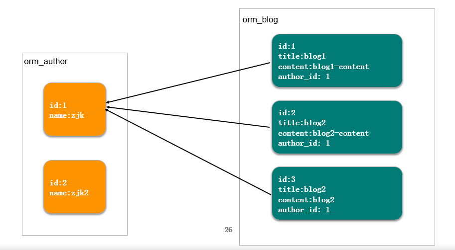
defwith_blog_counts(self, **kwargs): from django.db import connection cursor = connection.cursor() condition = '' if kwargs.has_key('id'): condition = 'a.id = %s and ' % kwargs['id'] query = ''' SELECT a.id, a.name, COUNT(b.id) FROM orm_author a LEFT JOIN orm_blog b ON a.id = b.author_id WHERE %s TRUE GROUP BY a.id ''' % condition
cursor.execute(query) result_list = [] for row in cursor.fetchall(): author = self.model(id=row[0], name=row[1]) author.blog_count = row[2] result_list.append(author) return result_list
classAuthor(models.Model): name = models.CharField(max_length=50) objects = AuthorManager()
authors = Author.objects.with_blog_counts(id=2) for author in authors: print author.name, author.blog_count
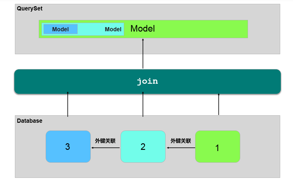
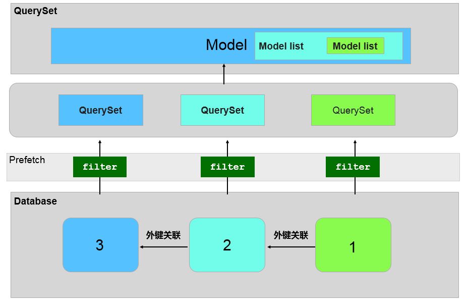
author = Author.objects.prefetch_related('blog_set').filter(name='zjk').first() for blog in author.blog_set.all(): print blog
# SQL: # SELECT `orm_author`.`id`, `orm_author`.`name` FROM `orm_author` # WHERE `orm_author`.`name` = 'zjk' ORDER BY `orm_author`.`id` ASC LIMIT 1 # # SELECT `orm_blog`.`id`, `orm_blog`.`author_id`, `orm_blog`.`title`, `orm_blog`.`content` # FROM `orm_blog` WHERE `orm_blog`.`author_id` IN (1)
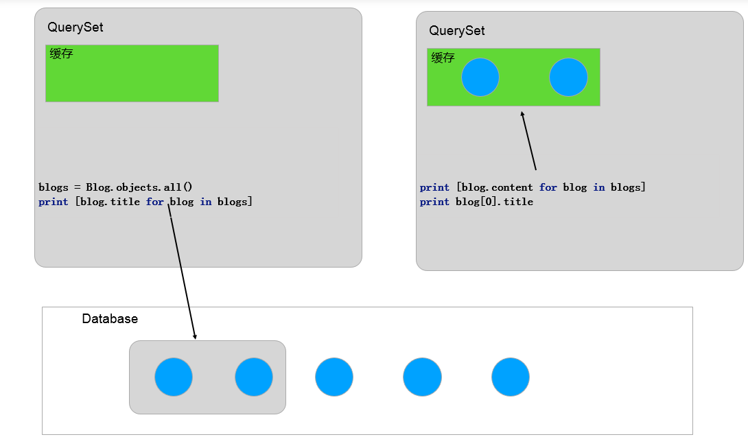
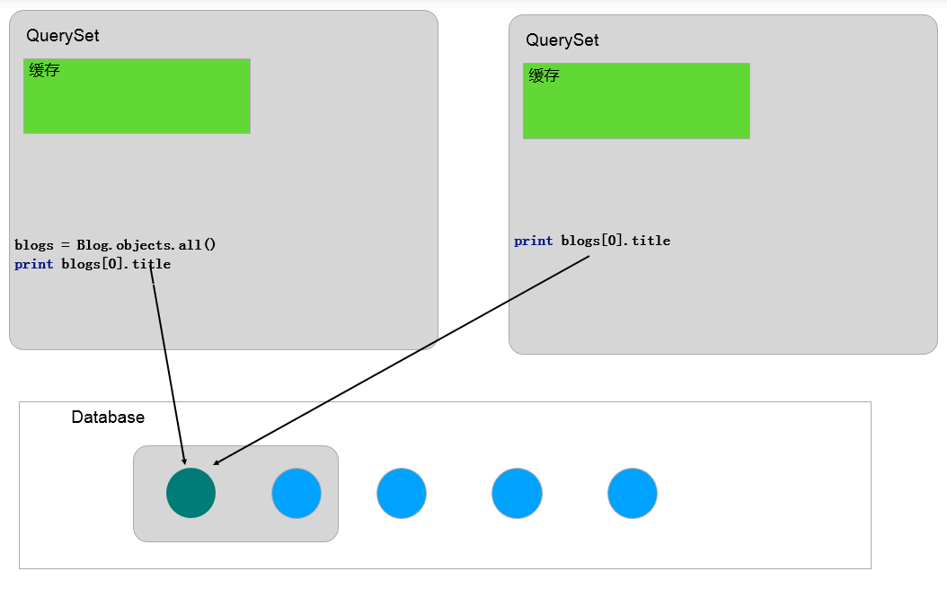
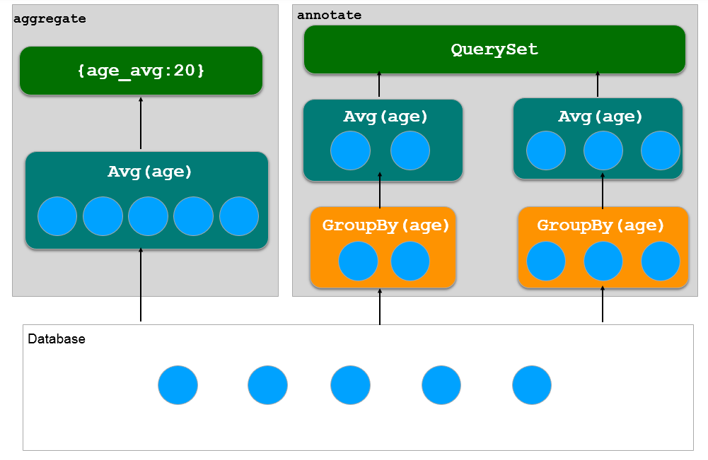
#认按照 id 进行分组 blogs = Blog.objects.annotate(Count('title')) for blog in blogs: print blog.title__count
# SELECT `orm_blog`.`id`, `orm_blog`.`author_id`, `orm_blog`.`title`, `orm_blog`.`content`, # COUNT(`orm_blog`.`title`) AS `title__count` FROM `orm_blog` GROUP BY `orm_blog`.`id` ORDER BY NULL
# 使用 values 方法,会按照 values 中传入的属性分组 blogs = Blog.objects.values('title').annotate(Count('title')) for blog in blogs: print blog['title__count']
# SELECT `orm_blog`.`title`, COUNT(`orm_blog`.`title`) AS `title__count` FROM `orm_blog` # GROUP BY `orm_blog`.`title` ORDER BY NULL
blogs = Blog.objects.values('title', 'content').annotate(Count('title')) for blog in blogs: print blog['title__count']
# SELECT `orm_blog`.`title`, `orm_blog`.`content`, COUNT(`orm_blog`.`title`) AS `title__count` # FROM `orm_blog` GROUP BY `orm_blog`.`title`, `orm_blog`.`content` ORDER BY NULL
下图是 aggregate 和 annotate 的比较:
extra
如何一些查询比较复杂可以考虑使用 extra 方法。extra 能在 ORM 生成的 SQL 子句中注入 SQL 代码,语法格式如下:
# - 表示倒序 blogs = Blog.objects.extra( order_by=['-id', 'title'] ) # SELECT . . . . . . FROM `orm_blog` ORDER BY `orm_blog`.`id` DESC, `orm_blog`.`title` ASC
原始 SQL 查询
使用 Manager 的 raw 方法可以用于原始的 SQL 查询,并返回 Model 的实例:
1 2 3
blogs = Blog.objects.raw('select * from orm_blog') for blog in blogs: print blog.id , blog.title
如果 SQL 中没有获取某个字段,那么会惰性加载该字段
1 2 3 4 5 6 7 8 9 10
# 没有取 title,在后面使用时会访问数据库 blogs = Blog.objects.raw('select id from orm_blog') for blog in blogs: print blog.id print blog.title
# select id from orm_blog # SELECT `orm_blog`.`id`, `orm_blog`.`title` FROM `orm_blog` WHERE `orm_blog`.`id` = 3 # SELECT `orm_blog`.`id`, `orm_blog`.`title` FROM `orm_blog` WHERE `orm_blog`.`id` = 4 #. . . .
一些优化
如果只需要判断实例是否存在,使用 exists 更高效
1 2 3 4 5
blogs = Blog.objects.filter(id=5) if blogs.exists(): print'record exist’ # SELECT (1) AS `a` FROM `orm_blog` WHERE `orm_blog`.`id` = 5 LIMIT 1
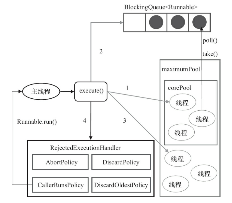
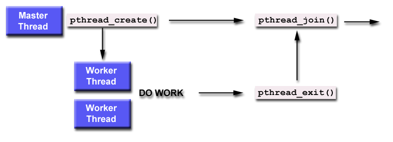
publicstaticvoidmain(String[] args){ ExecutorService executor = Executors.newFixedThreadPool(5); for (int i = 0; i < 10; i++) {
Runnable work = new WorkThread("" + i); executor.execute(work); } executor.shutdown(); while (!executor.isTerminated()) { } System.out.println("Finish all threads."); } }
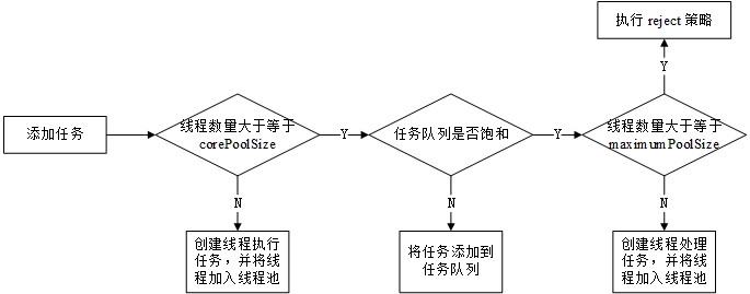
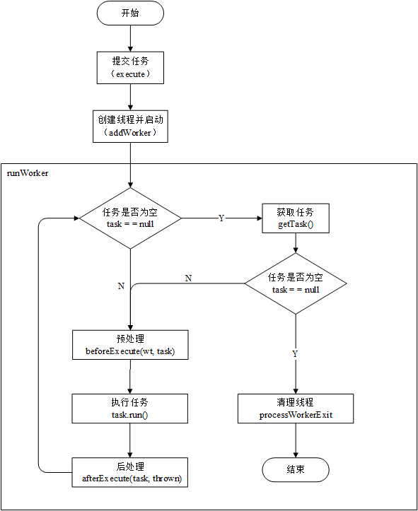
int c = ctl.get(); // 线程数量少于 corePoolSize,会创建一个新的线程执行该任务 if (workerCountOf(c) < corePoolSize) { // true 表示当前添加的线程为核心线程 if (addWorker(command, true)) return; c = ctl.get(); }
for (;;) { int wc = workerCountOf(c); // 线程数量大于系统规定的最大线程数或者大于 corePoolSize/maximumPoolSize // 表明线程池中无法添加新的线程,这里 wc >= CAPACITY 为了防止 corePoolSize // 或者 maximumPoolSize 大于CAPACITY if (wc >= CAPACITY || wc >= (core ? corePoolSize : maximumPoolSize)) { returnfalse; } // 使用 CAS 方式将线程数量增加,如果成功就跳出 retry if (compareAndIncrementWorkerCount(c)) { break retry; }
c = ctl.get(); // Re-read ctl // 如果线程池运行状态发生了改变就从 retry(外层循环)处重新开始, if (runStateOf(c) != rs) continue retry;
// 程序执行到这里说 CAS 没有成功,那么就再次执行 CAS } }
boolean workerStarted = false; boolean workerAdded = false; Worker w = null; try { // 创建 work w = new Worker(firstTask); final Thread t = w.thread; // t != null 说明线程创建成功了 if (t != null) { // 程序用一个 HashSet 存储线程,而 HashSet 不是线程的安全的, // 所以将线程加入 HashSet 的过程需要加锁。 final ReentrantLock mainLock = this.mainLock; mainLock.lock(); try { // Recheck while holding lock. // Back out on ThreadFactory failure or if // shut down before lock acquired. int rs = runStateOf(ctl.get());
// 1. rs < SHUTDOWN 说明程序在运行状态 // 2. rs == SHUTDOWN 说明当前线程处于平缓关闭状态,而 firstTask == null // 说明当前创建的线程是为了处理任务队列中剩余的任务(故意传入 null) if (rs < SHUTDOWN || (rs == SHUTDOWN && firstTask == null)) { // 线程是存活状态说明线程提前开始了。 if (t.isAlive()) // precheck that t is startable thrownew IllegalThreadStateException(); workers.add(w); int s = workers.size(); if (s > largestPoolSize) largestPoolSize = s; workerAdded = true; } } finally { mainLock.unlock(); } if (workerAdded) { // 启动线程 t.start(); workerStarted = true; } } } finally { if (!workerStarted) addWorkerFailed(w); } return workerStarted; }
队列同步器 AbstractQueuedSynchronizer(以下简称 AQS),是用来构建锁或者其他同步组件的基础框架。它使用一个 int 成员变量来表示同步状态,通过 CAS 操作对同步状态进行修改,确保状态的改变是安全的。通过内置的 FIFO (First In First Out)队列来完成资源获取线程的排队工作。更多关于 Java 多线程的文章可以转到 这里
publicstaticvoidwithoutMutex()throws InterruptedException { System.out.println("Without mutex: "); int threadCount = 2; final Thread threads[] = new Thread[threadCount]; for (int i = 0; i < threads.length; i++) { finalint index = i; threads[i] = new Thread(new Runnable() { @Override publicvoidrun(){ for (int j = 0; j < 100000; j++) { if (j % 20000 == 0) { System.out.println("Thread-" + index + ": j =" + j); } } } }); }
for (int i = 0; i < threads.length; i++) { threads[i].start(); } for (int i = 0; i < threads.length; i++) { threads[i].join(); } }
publicstaticvoidwithMutex(){ System.out.println("With mutex: "); final Mutex mutex = new Mutex(); int threadCount = 2; final Thread threads[] = new Thread[threadCount]; for (int i = 0; i < threads.length; i++) { finalint index = i; threads[i] = new Thread(new Runnable() {
下面在看一个共享锁的示例。在该示例中,我们定义两个共享资源,即同一时间内允许两个线程同时执行。我们将同步变量的初始状态 state 设为 2,当一个线程获取了共享锁之后,将 state 减 1,线程释放了共享锁后,将 state 加 1。状态的合法范围是 0、1 和 2,其中 0 表示已经资源已经用光了,此时线程再要获得共享锁就需要进入同步序列等待。下面是具体实现:
publicSync(int resourceCount){ if (resourceCount <= 0) { thrownew IllegalArgumentException("resourceCount must be larger than zero."); } // 设置可以共享的资源总数 setState(resourceCount); }
@Override protectedinttryAcquireShared(int reduceCount){ // 使用尝试获得资源,如果成功修改了状态变量(获得了资源) // 或者资源的总量小于 0(没有资源了),则返回。 for (; ; ) { int lastCount = getState(); int newCount = lastCount - reduceCount; if (newCount < 0 || compareAndSetState(lastCount, newCount)) { return newCount; } } }
@Override protectedbooleantryReleaseShared(int returnCount){ // 释放共享资源,因为可能有多个线程同时执行,所以需要使用 CAS 操作来修改资源总数。 for (; ; ) { int lastCount = getState(); int newCount = lastCount + returnCount; if (compareAndSetState(lastCount, newCount)) { returntrue; } } } }
// 定义两个共享资源,说明同一时间内可以有两个线程同时运行 privatefinal Sync sync = new Sync(2);
在上面的流程中,其实涉及到了两个操作,比较以及替换,为了确保程序正确,需要确保这两个操作的原子性(也就是说确保这两个操作同时进行,中间不会有其他线程干扰)。现在的 CPU 中,提供了相关的底层 CAS 指令,即 CPU 底层指令确保了比较和交换两个操作作为一个原子操作进行(其实在这一点上还是有排他锁的. 只是比起用synchronized, 这里的排他时间要短的多.),Java 中的 CAS 函数是借助于底层的 CAS 指令来实现的。更多关于 CPU 底层实现的原理可以参考 这篇文章。我们来看下 Java 中对于 CAS 函数的定义:
/** * Atomically update Java variable to x if it is currently * holding expected. * @return true if successful */ publicfinalnativebooleancompareAndSwapObject(Object o, long offset, Object expected, Object x);
/** * Atomically update Java variable to x if it is currently * holding expected. * @return true if successful */ publicfinalnativebooleancompareAndSwapInt(Object o, long offset, int expected, int x);
/** * Atomically update Java variable to x if it is currently * holding expected. * @return true if successful */ publicfinalnativebooleancompareAndSwapLong(Object o, long offset, long expected, long x);
上面三个函数定义在 sun.misc.Unsafe 类中,使用该类可以进行一些底层的操作,例如直接操作原生内存,更多关于 Unsafe 类的文章可以参考 这篇。以 compareAndSwapInt 为例,我们看下如何使用 CAS 函数:
/** * Report the location of a given static field, in conjunction with {@link * #staticFieldBase}. * Do not expect to perform any sort of arithmetic on this offset; * it is just a cookie which is passed to the unsafe heap memory accessors. * * Any given field will always have the same offset, and no two distinct * fields of the same class will ever have the same offset. * * As of 1.4.1, offsets for fields are represented as long values, * although the Sun JVM does not use the most significant 32 bits. * It is hard to imagine a JVM technology which needs more than * a few bits to encode an offset within a non-array object, * However, for consistency with other methods in this class, * this method reports its result as a long value. */ publicnativelongobjectFieldOffset(Field f);
下面我们再看一下 compareAndSwapInt 的函数原型。我们知道 CAS 操作需要知道 3 个信息:内存中的值,期望的旧值以及要修改的新值。通过前面的分析,我们知道通过 o 和 offset 我们可以确定属性在内存中的地址,也就是知道了属性在内存中的值。expected 对应期望的旧址,而 x 就是要修改的新值。
1
publicfinalnativebooleancompareAndSwapInt(Object o, long offset, int expected, int x);
compareAndSwapInt 函数首先比较一下 expected 是否和内存中的值相同,如果不同证明其他线程修改了属性值,那么就不会执行更新操作,但是程序如果就此返回了,似乎不太符合我们的期望,我们是希望程序可以执行更新操作的,如果其他线程先进行了更新,那么就在更新后的值的基础上进行修改,所以我们一般使用循环配合 CAS 函数,使程序在更新操作完成之后再返回,如下所示:
1 2 3 4
long before = counter; while (!unsafe.compareAndSwapLong(this, offset, before, before + 1)) { before = counter; }
publicvoidincrement(){ long before = counter; while (!unsafe.compareAndSwapLong(this, offset, before, before + 1)) { before = counter; } }
publiclonggetCounter(){ return counter; }
privatestaticlong intCounter = 0;
publicstaticvoidmain(String[] args)throws InterruptedException { int threadCount = 10; Thread threads[] = new Thread[threadCount]; final CASCounter casCounter = new CASCounter();
for (int i = 0; i < threadCount; i++) { threads[i] = new Thread(new Runnable() { @Override publicvoidrun(){
for (int i = 0; i < 10000; i++) { casCounter.increment(); intCounter++; } } }); threads[i].start(); }
for(int i = 0; i < threadCount; i++) { threads[i].join(); } System.out.printf("CASCounter is %d \nintCounter is %d\n", casCounter.getCounter(), intCounter); } }
PROPAGATE: -3,在共享模式下,可以认为资源有多个,因此当前线程被唤醒之后,可能还有剩余的资源可以唤醒其他线程。该状态用来表明后续节点会传播唤醒的操作。需要注意的是只有头节点才可以设置为该状态(This is set (for head node only) in doReleaseShared to ensure propagation continues, even if other operations have since intervened.)。
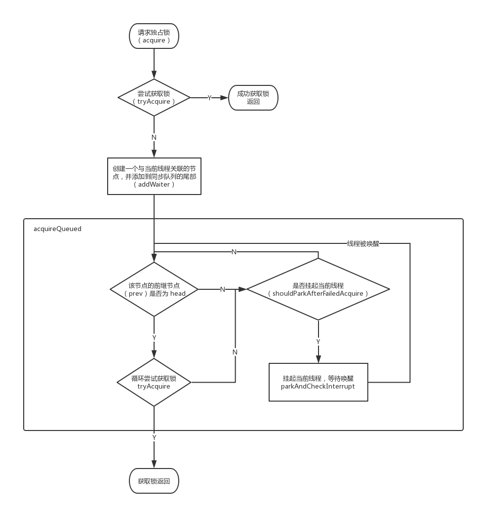
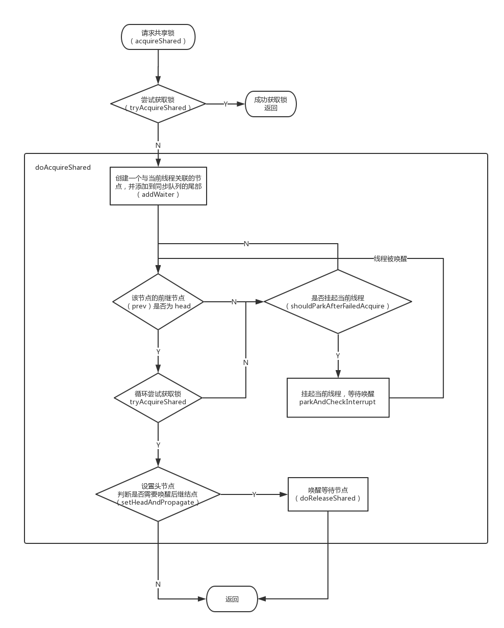
privatestaticbooleanshouldParkAfterFailedAcquire(Node pred, Node node){ // 当前节点的前继节点的等待状态 int ws = pred.waitStatus; // 如果前继节点的等待状态为 SIGNAL 我们就可以将当前节点对应的线程挂起 if (ws == Node.SIGNAL) returntrue; if (ws > 0) { // ws 大于 0,表明当前线程的前继节点处于 CANCELED 的状态, // 所以我们需要从当前节点开始往前查找,直到找到第一个不为 // CAECELED 状态的节点 do { node.prev = pred = pred.prev; } while (pred.waitStatus > 0); pred.next = node; } else { /* * waitStatus must be 0 or PROPAGATE. Indicate that we * need a signal, but don't park yet. Caller will need to * retry to make sure it cannot acquire before parking. */ compareAndSetWaitStatus(pred, ws, Node.SIGNAL); } returnfalse; }
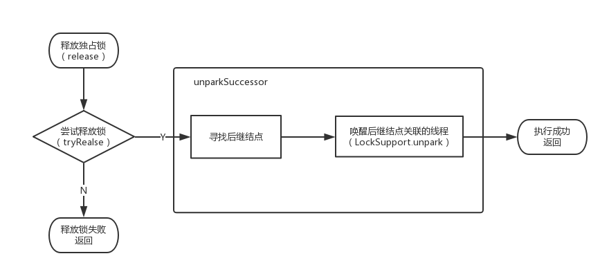
int ws = node.waitStatus; // 将 head 节点的状态置为 0,表明当前节点的后续节点已经被唤醒了, // 不需要再次唤醒,修改 ws 状态主要作用于 release 的判断 if (ws < 0) compareAndSetWaitStatus(node, ws, 0);
/* * Thread to unpark is held in successor, which is normally * just the next node. But if cancelled or apparently null, * traverse backwards from tail to find the actual * non-cancelled successor. */ Node s = node.next; if (s == null || s.waitStatus > 0) { s = null; for (Node t = tail; t != null && t != node; t = t.prev) if (t.waitStatus <= 0) s = t; } if (s != null) LockSupport.unpark(s.thread); }
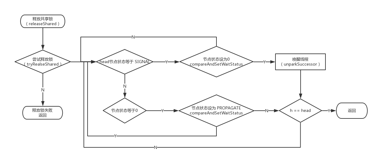
privatevoiddoReleaseShared(){ /* * Ensure that a release propagates, even if there are other * in-progress acquires/releases. This proceeds in the usual * way of trying to unparkSuccessor of head if it needs * signal. But if it does not, status is set to PROPAGATE to * ensure that upon release, propagation continues. * Additionally, we must loop in case a new node is added * while we are doing this. Also, unlike other uses of * unparkSuccessor, we need to know if CAS to reset status * fails, if so rechecking. */ for (;;) { Node h = head; // head = null 说明没有初始化,head = tail 说明同步队列中没有等待节点 if (h != null && h != tail) { // 查看当前节点的等待状态 int ws = h.waitStatus; // 我们在前面说过,SIGNAL说明有后续节点需要唤醒 if (ws == Node.SIGNAL) {
/* * 将当前节点的值设为 0,表明已经唤醒了后继节点 * 可能会有多个线程同时执行到这一步,所以使用 CAS 保证只有一个线程能修改成功, * 从而执行 unparkSuccessor,其他的线程会执行 continue 操作 */ if (!compareAndSetWaitStatus(h, Node.SIGNAL, 0)) continue; // loop to recheck cases unparkSuccessor(h); } elseif (ws == 0 && !compareAndSetWaitStatus(h, 0, Node.PROPAGATE)) { /* * ws 等于 0,说明无需唤醒后继结点(后续节点已经被唤醒或者当前节点没有被阻塞的后继结点), * 也就是这一次的调用其实并没有执行唤醒后继结点的操作。就类似于我只需要一张优惠券, * 但是我的两个朋友,他们分别给我了一张,因此我就剩余了一张。然后我就将这张剩余的优惠券 * 送(传播)给其他人使用,因此这里将节点置为可传播的状态(PROPAGATE) */ continue; // loop on failed CAS } } if (h == head) // loop if head changed break; } }
privatevoidsetHeadAndPropagate(Node node, long propagate){ // 备份一下头节点 Node h = head; // Record old head for check below /* * 移除头节点,并将当前节点置为头节点 * 当执行完这一步之后,其实队列的头节点已经发生改变, * 其他被唤醒的线程就有机会去获取锁,从而并发的执行该方法, * 所以上面备份头节点,以便下面的代码可以正确运行 */ setHead(node);
/* * Try to signal next queued node if: * Propagation was indicated by caller, * or was recorded (as h.waitStatus either before * or after setHead) by a previous operation * (note: this uses sign-check of waitStatus because * PROPAGATE status may transition to SIGNAL.) * and * The next node is waiting in shared mode, * or we don't know, because it appears null * * The conservatism in both of these checks may cause * unnecessary wake-ups, but only when there are multiple * racing acquires/releases, so most need signals now or soon * anyway. */
/* * 判断是否需要唤醒后继结点,propagate > 0 说明共享资源有剩余, * h.waitStatus < 0,表明当前节点状态可能为 SIGNAL,CONDITION,PROPAGATE */ if (propagate > 0 || h == null || h.waitStatus < 0 || (h = head) == null || h.waitStatus < 0) { Node s = node.next; // 只有 s 不处于独占模式时,才去唤醒后继结点 if (s == null || s.isShared()) doReleaseShared(); } }
到了这里,脉络就比较清晰了,当一个节点获取到共享锁之后,它除了将自身设为 head 节点之外,还会判断一下是否满足唤醒后继结点的条件,如果满足,就唤醒后继结点,后继结点获取到锁之后,会重复这个过程,直到判断条件不成立。就类似于考试时从第一排往最后一排传卷子,第一排先留下一份,然后将剩余的传给后一排,后一排会重复这个过程。如果传到某一排卷子没了,那么位于这排的人就要等待,直到老师又给了他新的卷子。
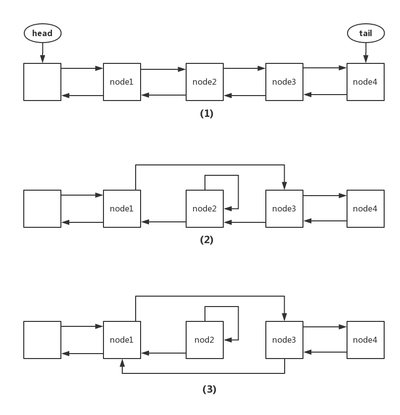
privatevoidcancelAcquire(Node node){ // Ignore if node doesn't exist if (node == null) return;
node.thread = null;
// 跳过前面的已经取消的节点 Node pred = node.prev; while (pred.waitStatus > 0) node.prev = pred = pred.prev;
// 保存下 pred 的后继结点,以便 CAS 操作使用 // 因为可能存在已经取消的节点,所以 pred.next 不一等于 node Node predNext = pred.next;
// Can use unconditional write instead of CAS here. // After this atomic step, other Nodes can skip past us. // Before, we are free of interference from other threads. // 将节点状态设为 CANCELED node.waitStatus = Node.CANCELLED;
// If we are the tail, remove ourselves. if (node == tail && compareAndSetTail(node, pred)) { compareAndSetNext(pred, predNext, null); } else { // If successor needs signal, try to set pred's next-link // so it will get one. Otherwise wake it up to propagate. int ws; if (pred != head && ((ws = pred.waitStatus) == Node.SIGNAL || (ws <= 0 && compareAndSetWaitStatus(pred, ws, Node.SIGNAL))) && pred.thread != null) { Node next = node.next; if (next != null && next.waitStatus <= 0) compareAndSetNext(pred, predNext, next); } else { unparkSuccessor(node); }
在上面的代码中,increase 线程和 decrease 线程会操作同一个 number 中 value,那么输出的结果是不可预测的,因为当前线程修改变量之后但是还没输出的时候,变量有可能被另外一个线程修改,下面是一种可能的情况:
1 2
increase value: 10 decrease value: 10
一种解决方法是在 increase() 和 decrease() 方法上加上 synchronized 关键字进行同步,这种做法其实是将 value 的 赋值 和 打印 包装成了一个原子操作,也就是说两者要么同时进行,要不都不进行,中间不会有额外的操作。我们换个角度考虑问题,如果 value 只属于 increase 线程或者 decrease 线程,而不是被两个线程共享,那么也不会出现竞争问题。一种比较常见的形式就是局部(local)变量(这里排除局部变量引用指向共享对象的情况),如下所示:
1 2 3 4 5
publicvoidincrease()throws InterruptedException { int value = 10; Thread.sleep(10); System.out.println("increase value: " + value); }
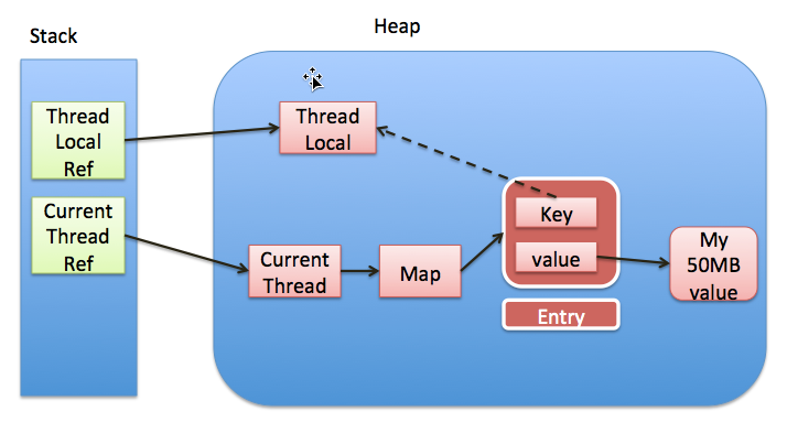
不论 value 值如何改变,都不会影响到其他线程,因为在每次调用 increase 方法时,都会创建一个 value 变量,该变量只对当前调用 increase 方法的线程可见。借助于这种思想,我们可以对每个线程创建一个共享变量的副本,该副本只对当前线程可见(可以认为是线程私有的变量),那么修改该副本变量时就不会影响到其他的线程。一个简单的思路是使用 Map 存储每个变量的副本,将当前线程的 id 作为 key,副本变量作为 value 值,下面是一个实现:
每个线程对应的副本变量的生命周期不是由线程决定的,而是由共享变量的生命周期决定的。在上面的例子中,即便线程执行完,只要 number 变量存在,线程的副本变量依然会存在(存放在 number 的 cacheMap 中)。但是作为特定线程的副本变量,该变量的生命周期应该由线程决定,线程消亡之后,该变量也应该被回收。
// We don't use a fast path as with get() because it is at // least as common to use set() to create new entries as // it is to replace existing ones, in which case, a fast // path would fail more often than not.
Entry[] tab = table; int len = tab.length; // 根据 ThreadLocal 的散列值,查找对应元素在数组中的位置 int i = key.threadLocalHashCode & (len - 1);
// 使用线性探测法查找元素 for (Entry e = tab[i]; e != null; e = tab[i = nextIndex(i, len)]) { ThreadLocal <?> k = e.get(); // ThreadLocal 对应的 key 存在,直接覆盖之前的值 if (k == key) { e.value = value; return; } // key为 null,但是值不为 null,说明之前的 ThreadLocal 对象已经被回收了,当前数组中的 Entry 是一个陈旧(stale)的元素 if (k == null) { // 用新元素替换陈旧的元素,这个方法进行了不少的垃圾清理动作,防止内存泄漏,具体可以看源代码,没看太懂 replaceStaleEntry(key, value, i); return; } } // ThreadLocal 对应的 key 不存在并且没有找到陈旧的元素,则在空元素的位置创建一个新的 Entry。 tab[i] = new Entry(key, value); int sz = ++size; // cleanSomeSlot 清理陈旧的 Entry(key == null),具体的参考源码。如果没有清理陈旧的 Entry 并且数组中的元素大于了阈值,则进行 rehash。 if (!cleanSomeSlots(i, sz) && sz >= threshold) rehash(); }
关于 set 方法,有几点需要地方:
int i = key.threadLocalHashCode & (len - 1);,这里实际上是对 len-1 进行了取余操作。之所以能这样取余是因为 len 的值比较特殊,是 2 的 n 次方,减 1 之后低位变为全 1,高位变为全 0。例如 16,减 1 之后对应的二进制为: 00001111,这样其他数字中大于 16 的部分就会被 0 与掉,小于 16 的部分就会保留下来,就相当于取余了。
private Entry getEntryAfterMiss(ThreadLocal <?> key, int i, Entry e){ Entry[] tab = table; int len = tab.length;
while (e != null) { ThreadLocal < ? > k = e.get(); if (k == key) return e; if (k == null) expungeStaleEntry(i); else i = nextIndex(i, len); e = tab[i]; } returnnull; }
privatevoidremove(ThreadLocal <?> key){ Entry[] tab = table; int len = tab.length; int i = key.threadLocalHashCode & (len - 1); for (Entry e = tab[i]; e != null; e = tab[i = nextIndex(i, len)]) { if (e.get() == key) { e.clear(); expungeStaleEntry(i); return; } } }
副本变量存取
前面说完了 ThreadLocalMap,副本变量的存取操作就很好理解了。下面是 ThreadLocal 中的 set 和 get 方法的实现:
publicvoidset(T value){ Thread t = Thread.currentThread(); ThreadLocalMap map = getMap(t); if (map != null) map.set(this, value); else createMap(t, value); }
public T get(){ Thread t = Thread.currentThread(); ThreadLocalMap map = getMap(t); if (map != null) { ThreadLocalMap.Entry e = map.getEntry(this); if (e != null) { @SuppressWarnings("unchecked") T result = (T) e.value; return result; } } return setInitialValue(); }
/** * ThreadLocals rely on per-thread linear-probe hash maps attached * to each thread (Thread.threadLocals and * inheritableThreadLocals). The ThreadLocal objects act as keys, * searched via threadLocalHashCode. This is a custom hash code * (useful only within ThreadLocalMaps) that eliminates collisions * in the common case where consecutively constructed ThreadLocals * are used by the same threads, while remaining well-behaved in * less common cases. */ privatefinalint threadLocalHashCode = nextHashCode();
/** * The next hash code to be given out. Updated atomically. Starts at * zero. */ privatestatic AtomicInteger nextHashCode = new AtomicInteger();
/** * The difference between successively generated hash codes - turns * implicit sequential thread-local IDs into near-optimally spread * multiplicative hash values for power-of-two-sized tables. */ privatestaticfinalint HASH_INCREMENT = 0x61c88647;
/** * Returns the next hash code. */ privatestaticintnextHashCode(){ return nextHashCode.getAndAdd(HASH_INCREMENT); }
// 读取选择或者拖拽的文件(多个文件) functionprocessImages(imgFiles) { var index = 0; for (i = 0; i < imgFiles.length; i++) { var file = imgFiles[i]; var reader = new FileReader(); reader.readAsDataURL(file); (function (reader, file) { reader.onload = function (e) { cacheImages[file.name] = e.target.result; index++; if (index == length) { replaceImage(); } } })(reader, file); } }
// 将路径替换为图片内容 functionreplaceImage() { var images = $("img"); var i; for (i = 0; i < images.length; i++) { var imgSrc = images[i].src; var imgName = getImgName(imgSrc); if (cacheImages.hasOwnProperty(imgName)) { images[i].src = cacheImages[imgName]; } } }
// resize the canvas and draw the image data into it canvas.width = width; canvas.height = height; var ctx = canvas.getContext("2d"); ctx.drawImage(img, 0, 0, width, height); return canvas.toDataURL(format); }
循环中使用异步回调函数
为了方便使用,我们可以同时上传多个图片,我们使用 for 循环来读取多个文件,但是有个问题是文件的读取是异步的,也就是说在 for 循环执行完之后,图片可能仍在读取中,当图片读取完后,再调用 onload 回调函数进行处理。简单一点就是说如何在 for 循环中正确使用延迟调用的回调函数。看下面的例子:
1 2 3 4 5 6 7 8 9 10 11
functionprint(value, callback) { console.log("value in print", value); setTimeout(callback, 1000); }
for(var i = 0; i < 4; i++) { var value = i; print(value, function() { console.log("value in callback", value); }); }
<scriptsrc="http://cdn.bootcss.com/emojify.js/1.1.0/js/emojify.min.js"></script> <scripttype="text/javascript"> trueemojify.setConfig({ emojify_tag_type: 'div', // Only run emojify.js on this element only_crawl_id: null, // Use to restrict where emojify.js applies img_dir: 'http://cdn.bootcss.com/emojify.js/1.0/images/basic', // Directory for emoji images ignored_tags: { // Ignore the following tags 'SCRIPT': 1, 'TEXTAREA': 1, 'A': 1, 'PRE': 1, 'CODE': 1 } }); </script>
将 markdown 文件转为 html 之后,调用 emojify 中的方法将对应标记转换 emoji 表情。
// 触发事件 fire: function (type, event) { if (event == null || event.type == null) { return; }
if (this._listeners[event.type] instanceofArray) { var listeners = this._listeners[event.type]; for (var i = 0, len = listeners.length; i < len; i++) { listeners[i].call(this, event); } } },
// 如果listener 为null,则清除当前事件下的全部事件监听 removeListener: function (type, listener) { if (listener == null) { if (this._listeners.hasOwnProperty(type)) { this._listeners[type] = []; cce.EventManager.removeTarget(type, this); } } if (this._listeners[type] instanceofArray) { var listeners = this._listeners[type]; for (var i = 0, len = listeners.length; i < len; i++) { if (listeners[i] === listener) { listeners.splice(i, 1); if (listeners.length == 0) cce.EventManager.removeTarget(type, this); break; } } }
在判断触发某个事件的元素时,需要遍历所有绑定了该事件的元素,判断鼠标位置是否位于元素内部。为了减少不必要的比较,这里使用了一个有序数组,使用元素区域的最小 x 值作为比较值,按照升序排列。如果一个元素区域的最小 x 值大于鼠标的 x 值,那么就无需比较数组中该元素后面的元素。具体实现可以看 SortArray.js
// 在有序数组中会根据这个方法的返回结果将对象排序 cce.DisplayObject.prototype.compareTo = function (target) { returnnull; };
// 比较目标点的x值与当前区域的最小 x 值,结合有序数组使用,如果 point 的 x 小于当前区域的最小 x 值,那么有序数组中剩余 // 元素的最小 x 值也会大于目标点的 x 值,就可以停止比较。在事件判断时首先使用该函数过滤一下。 cce.DisplayObject.prototype.comparePointX = function (point) { returnnull; };
// 判断目标点是否在当前区域内 cce.DisplayObject.prototype.hasPoint = function (point) { returnfalse; };
if(myObj.hasOwnProperty("<property name>")){ alert("yes, i have that property"); } // 或者 if("<property name>"in myObj) { alert("yes, i have that property"); }
The float CSS property specifies that an element should be taken from the normal flow and placed along the left or right side of its container, where text and inline elements will wrap around it.
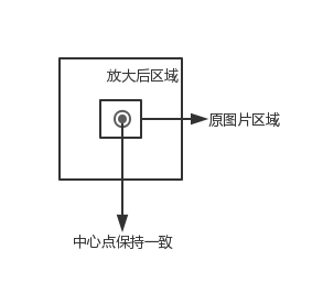
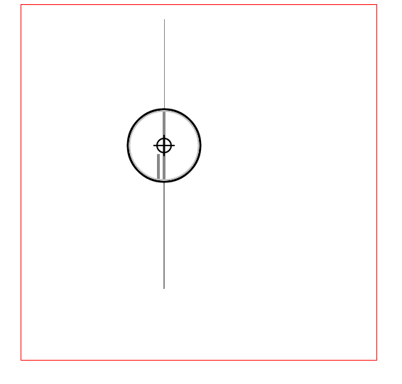
// 原始线段 var chartLines = newArray(); // 处于放大镜中的原始线段 var glassLines; // 放大后的线段 var scaleGlassLines; // 位于放大镜中的线段数量 var glassLineSize;
functioninitLines() {
var line; line = new Line(200.5, 400, 200.5, 200, 0, "#888"); chartLines.push(line); line = new Line(201.5, 400, 201.5, 20, 1, "#888"); chartLines.push(line);
glassLineSize = chartLines.length; glassLines = newArray(glassLineSize); for (var i = 0; i < glassLineSize; i++) { line = new Line(0, 0, 0, 0, i); glassLines[i] = line; }
scaleGlassLines = newArray(glassLineSize); for (var i = 0; i < glassLineSize; i++) { line = new Line(0, 0, 0, 0, i); scaleGlassLines[i] = line; } }
绘制线段
1 2 3 4 5 6 7 8 9 10 11 12 13
functiondrawLines() { var line; context.lineWidth = 1;
for (var i = 0; i < chartLines.length; i++) { line = chartLines[i]; context.beginPath(); context.strokeStyle = line.color; context.moveTo(line.xStart, line.yStart); context.lineTo(line.xEnd, line.yEnd); context.stroke(); } }
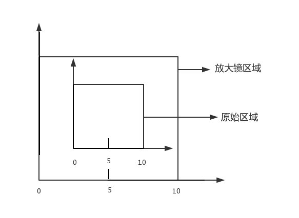
functioncalScaleLines() { var xStart = originalRectangle.x; var xEnd = originalRectangle.x + originalRectangle.width; var yStart = originalRectangle.y; var yEnd = originalRectangle.y + originalRectangle.height; var line, gLine, sgLine; var glassLineIndex = 0; for (var i = 0; i < chartLines.length; i++) { line = chartLines[i];
for (var i = 0; i < chartLines.length; i++) { var line = chartLines[i]; if (line.index == index) { line.color = "#f00"; } else { line.color = "#888"; } }
draw(); }
键盘事件
因为线段离得比较近,所以使用鼠标移动很难精确的选中线段,这里使用键盘的w, a, s, d 来进行精确移动
1 2 3 4 5 6 7 8 9 10 11 12 13 14 15
document.onkeyup = function (e) { if (e.key == 'w') { centerPoint.y = intAdd(centerPoint.y, -0.2); } if (e.key == 'a') { centerPoint.x = intAdd(centerPoint.x, -0.2); } if (e.key == 's') { centerPoint.y = intAdd(centerPoint.y, 0.2); } if (e.key == 'd') { centerPoint.x = intAdd(centerPoint.x, 0.2); } draw(); }
Specifies the buffer to be used by the stream for I/O operations, which becomes a fully buffered stream. Or, alternatively, if buffer is a null pointer, buffering is disabled for the stream, which becomes an unbuffered stream.
On output, data is written once the buffer is full (or flushed). On Input, the buffer is filled when an input operation is requested and the buffer is empty.
On output, data is written when a newline character is inserted into the stream or when the buffer is full (or flushed), whatever happens first. On Input, the buffer is filled up to the next newline character when an input operation is requested and the buffer is empty.
Information for data/test.txt --------------------------- File Size: 24023896 bytes Number of Links: 1 File inode: 8261278 File Permissions: -rw-rw-r--
任意一个并行域都不能嵌套在其他并行域中(Neither parallel region is nested inside another explicit parallel region.)
执行两个并行域的线程数量要相同(The number of threads used to execute both parallel regions is the same.)
执行两个并行域时的线程亲和度策略要相同( The thread affinity policies used to execute both parallel regions are the same.)
在进入并行域之前dyn-var变量的值必须为false(0). (The value of the dyn-var internal control variable in the enclosing task region is false at entry to both parallel regions.)
int counter = 10; #pragma omp threadprivate(counter)
voidtest_copyprivate(){ int i; #pragma omp parallel private(i) { #pragma omp single copyprivate(i, counter) { i = 50; counter = 100; printf("thread %d execute single\n", omp_get_thread_num()); } printf("thread %d: i is %d and counter is %d\n",omp_get_thread_num(), i, counter);
} }
下面是程序运行结果:
1 2 3 4 5
thread 3 execute single thread 2: i is 50 and counter is 100 thread 3: i is 50 and counter is 100 thread 0: i is 50 and counter is 100 thread 1: i is 50 and counter is 100
下面是将copyprivate(i, counter)去掉的运行结果
1 2 3 4 5
thread 0 execute single thread 2: i is 0 and counter is 10 thread 0: i is 50 and counter is 100 thread 3: i is 0 and counter is 10 thread 1: i is 32750 and counter is 10
voidtest_numthread(){ printf("max thread nums is %d\n", omp_get_max_threads()); printf("omp_get_num_threads: out parallel region is %d\n", omp_get_num_threads()); omp_set_num_threads(2); printf("after omp_set_num_threads: max thread nums is %d\n", omp_get_max_threads()); #pragma omp parallel { #pragma omp master { printf("omp_get_num_threads: in parallel region is %d\n\n", omp_get_num_threads()); } printf("1: thread %d is running\n", omp_get_thread_num()); } printf("\n"); #pragma omp parallel num_threads(3) { printf("2: thread %d is running\n", omp_get_thread_num()); } }
下面是程序运行结果:
1 2 3 4 5 6 7 8 9 10 11
max thread nums is 4 omp_get_num_threads: out parallel region is 1 after omp_set_num_threads: max thread nums is 2 omp_get_num_threads: in parallel region is 2
1: thread 0 is running 1: thread 1 is running
2: thread 0 is running 2: thread 1 is running 2: thread 2 is running
voidtest_nested(){ int tid; printf("nested state is %d\n", omp_get_nested());
#pragma omp parallel num_threads(2) private(tid) { tid = omp_get_thread_num(); printf("In outer parallel region: thread %d is running\n", tid); #pragma omp parallel num_threads(2) firstprivate(tid) { printf("In nested parallel region: thread %d is running and outer thread is %d\n", omp_get_thread_num(), tid); } }
omp_set_nested(1); printf("\n"); printf("nested state is %d\n", omp_get_nested());
#pragma omp parallel num_threads(2) private(tid) { tid = omp_get_thread_num(); printf("In outer parallel region: thread %d is running\n", tid); #pragma omp parallel num_threads(2) { printf("In nested parallel region: thread %d is running and outer thread is %d\n", omp_get_thread_num(), tid); } } }
下面是程序运行结果:
1 2 3 4 5 6 7 8 9 10 11 12 13
nested state is 0 In outer parallel region: thread 0 is running In nested parallel region: thread 0 is running and outer thread is 0 In outer parallel region: thread 1 is running In nested parallel region: thread 0 is running and outer thread is 1
nested state is 1 In outer parallel region: thread 1 is running In outer parallel region: thread 0 is running In nested parallel region: thread 0 is running and outer thread is 0 In nested parallel region: thread 0 is running and outer thread is 1 In nested parallel region: thread 1 is running and outer thread is 1 In nested parallel region: thread 1 is running and outer thread is 0
voidparallel_single(){ int a = 0, n = 10, i; int b[n]; #pragma omp parallel shared(a, b) private(i) { // 只有一个线程会执行这段代码, 其他线程会等待该线程执行完毕 #pragma omp single { a = 10; printf("Single construct executed by thread %d\n", omp_get_thread_num()); }
// A barrier is automatically inserted here #pragma omp for for(i = 0; i < n; i++) { b[i] = a; } }
printf("After the parallel region:\n"); for (i=0; i<n; i++) printf("b[%d] = %d\n",i,b[i]); }
下面是执行结果:
1 2 3 4 5 6 7 8 9 10 11 12
Single construct executed by thread 2 After the parallel region: b[0] = 10 b[1] = 10 b[2] = 10 b[3] = 10 b[4] = 10 b[5] = 10 b[6] = 10 b[7] = 10 b[8] = 10 b[9] = 10
下面是single指令后面可以跟随的子句:
1 2 3 4 5 6 7
private(list)
firstprivate(list)
copyprivate(list)
nowait
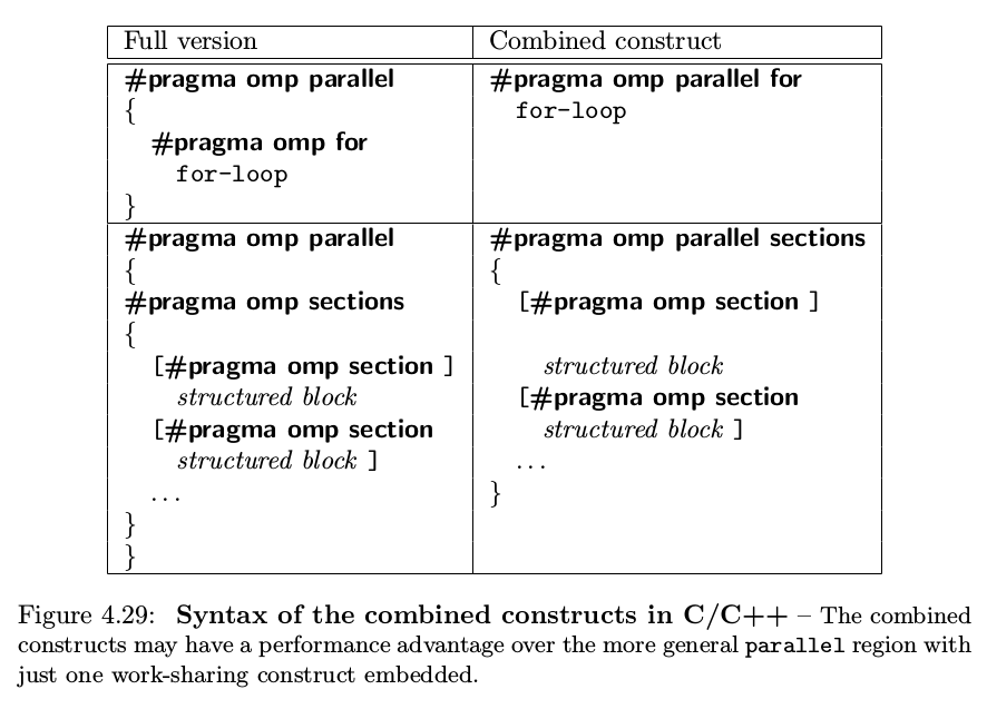
Combined Parallel Work-Sharing Constructs
将parallel指令和work-sharing指令结合起来, 使代码更加简洁. 如下面的代码
1 2 3 4 5
#pragma omp parallel { #pragma omp for for(.....) }
voidtest_private(){ int n = 8; int i=2, a = 3; // i,a 定义为private之后不改变原先的值 #pragma omp parallel for private(i, a) for ( i = 0; i<n; i++) { a = i+1; printf("In for: thread %d has a value of a = %d for i = %d\n", omp_get_thread_num(),a,i); }
printf("\n"); printf("Out for: thread %d has a value of a = %d for i = %d\n", omp_get_thread_num(),a,i); }
下面是程序运行结果:
1 2 3 4 5 6 7 8 9 10
In for: thread 2 has a value of a = 5 for i = 4 In for: thread 2 has a value of a = 6 for i = 5 In for: thread 3 has a value of a = 7 for i = 6 In for: thread 3 has a value of a = 8 for i = 7 In for: thread 0 has a value of a = 1 for i = 0 In for: thread 0 has a value of a = 2 for i = 1 In for: thread 1 has a value of a = 3 for i = 2 In for: thread 1 has a value of a = 4 for i = 3
voidtest_last_private(){ int n = 8; int i=2, a = 3; // lastprivate 将for中最后一次循环(i == n-1) a 的值赋给a #pragma omp parallel for private(i) lastprivate(a) for ( i = 0; i<n; i++) { a = i+1; printf("In for: thread %d has a value of a = %d for i = %d\n", omp_get_thread_num(),a,i); }
printf("\n"); printf("Out for: thread %d has a value of a = %d for i = %d\n", omp_get_thread_num(),a,i); }
程序执行结果为:
1 2 3 4 5 6 7 8 9 10
In for: thread 3 has a value of a = 7 for i = 6 In for: thread 3 has a value of a = 8 for i = 7 In for: thread 2 has a value of a = 5 for i = 4 In for: thread 2 has a value of a = 6 for i = 5 In for: thread 1 has a value of a = 3 for i = 2 In for: thread 0 has a value of a = 1 for i = 0 In for: thread 0 has a value of a = 2 for i = 1 In for: thread 1 has a value of a = 4 for i = 3
voidtest_first_private(){ int n = 8; int i=0, a[n];
for(i = 0; i < n ;i++) { a[i] = i+1; } #pragma omp parallel for private(i) firstprivate(a) for ( i = 0; i<n; i++) { printf("thread %d: a[%d] is %d\n", omp_get_thread_num(), i, a[i]); } }
执行结果如下:
1 2 3 4 5 6 7 8
thread 0: a[0] is 1 thread 0: a[1] is 2 thread 2: a[4] is 5 thread 2: a[5] is 6 thread 3: a[6] is 7 thread 3: a[7] is 8 thread 1: a[2] is 3 thread 1: a[3] is 4
Thread 3 before barrier at 16:55:44 Thread 2 before barrier at 16:55:44 Thread 3 after barrier at 16:55:44 Thread 2 after barrier at 16:55:44 Thread 1 before barrier at 16:55:47 Thread 0 before barrier at 16:55:47 Thread 0 after barrier at 16:55:47 Thread 1 after barrier at 16:55:47
下面上加上路障的输出结果:
1
2
3
4
5
6
7
8
Thread 3 before barrier at 17:05:29 Thread 2 before barrier at 17:05:29 Thread 0 before barrier at 17:05:32 Thread 1 before barrier at 17:05:32 Thread 0 after barrier at 17:05:32 Thread 1 after barrier at 17:05:32 Thread 2 after barrier at 17:05:32 Thread 3 after barrier at 17:05:32
Thread 2: sumLocal = 1550 sum =1550 Thread 3: sumLocal = 2175 sum =3725 Thread 1: sumLocal = 925 sum =4650 Thread 0: sumLocal = 300 sum =4950 Value of sum after parallel region: 4950
下面是将临界区去掉的运行结果(运行结果不是固定的, 这里只是其中一种情况):
1 2 3 4 5
Thread 2: sumLocal = 1550 sum =1550 Thread 3: sumLocal = 2175 sum =2475 Thread 1: sumLocal = 925 sum =925 Thread 0: sumLocal = 300 sum =300 Value of sum after parallel region: 2475
voidtest_master(){ int a, i, n = 5; int b[n]; #pragma omp parallel shared(a, b) private(i) { #pragma omp master { a = 10; printf("Master construct is executed by thread %d\n", omp_get_thread_num()); } #pragma omp barrier
#pragma omp for for(i = 0; i < n; i++) b[i] = a; }
printf("After the parallel region:\n"); for(i = 0; i < n; i++) printf("b[%d] = %d\n", i, b[i]); }
下面是输出结果
1 2 3 4 5 6 7
Master construct is executed by thread 0 After the parallel region: b[0] = 10 b[1] = 10 b[2] = 10 b[3] = 10 b[4] = 10